General Solution to a Nonhomogeneous Linear System of Ode's
We discuss theory related to nonhomogeneous linear equations.
Nonhomogeneous Linear Equations
We'll now consider the nonhomogeneous linear second order equation
where the forcing function isn't identically zero. The next theorem, an extension of Theorem thmtype:5.1.1, gives sufficient conditions for existence and uniqueness of solutions of initial value problems for (eq:5.3.1). We omit the proof, which is beyond the scope of this book.
Suppose , and are continuous on an open interval , let be any point in , and let and be arbitrary real numbers. Then the initial value problem has a unique solution on .
To find the general solution of (eq:5.3.1) on an interval where , , and are continuous, it's necessary to find the general solution of the associated homogeneous equation
on . We call (eq:5.3.2) the complementary equation for (eq:5.3.1).
The next theorem shows how to find the general solution of (eq:5.3.1) if we know one solution of (eq:5.3.1) and a fundamental set of solutions of (eq:5.3.2). We call a particular solution of (eq:5.3.1); it can be any solution that we can find, one way or another.
Suppose , , and are continuous on . Let be a particular solution of on , and let be a fundamental set of solutions of the complementary equation on . Then is a solution of on if and only if where and are constants.
- Proof
- We first show that in (eq:5.3.5) is a solution of (eq:5.3.3) for any choice of the constants and . Differentiating (eq:5.3.5) twice yields so since satisfies (eq:5.3.3) and and satisfy (eq:5.3.4).
Now we'll show that every solution of (eq:5.3.3) has the form (eq:5.3.5) for some choice of the constants and . Suppose is a solution of (eq:5.3.3). We'll show that is a solution of (eq:5.3.4), and therefore of the form , which implies (eq:5.3.5). To see this, we compute
since and both satisfy (eq:5.3.3).
We say that (eq:5.3.5) is the general solution of on .
If , , and are continuous and has no zeros on , then Theorem thmtype:5.3.2 implies that the general solution of
on is , where is a particular solution of (eq:5.3.6) on and is a fundamental set of solutions of on . To see this, we rewrite (eq:5.3.6) as and apply Theorem thmtype:5.3.2 with , , and .
To avoid awkward wording in examples and exercises, we won't specify the interval when we ask for the general solution of a specific linear second order equation, or for a fundamental set of solutions of a homogeneous linear second order equation. Let's agree that this always means that we want the general solution (or a fundamental set of solutions, as the case may be) on every open interval on which , , and are continuous if the equation is of the form (eq:5.3.3), or on which , , , and are continuous and has no zeros, if the equation is of the form (eq:5.3.6). We leave it to you to identify these intervals in specific examples and exercises.
For completeness, we point out that if , , , and are all continuous on an open interval , but does have a zero in , then (eq:5.3.6) may fail to have a general solution on in the sense just defined.
In this section we to limit ourselves to applications of Theorem thmtype:5.3.2 where we can guess at the form of the particular solution.
- (a)
- Find the general solution of
- (b)
- Solve the initial value problem
item:5.3.1a We can apply Theorem thmtype:5.3.2 with , since the functions , , and in (eq:5.3.7) are continuous on . By inspection we see that is a particular solution of (eq:5.3.7). Since and form a fundamental set of solutions of the complementary equation , the general solution of (eq:5.3.7) is
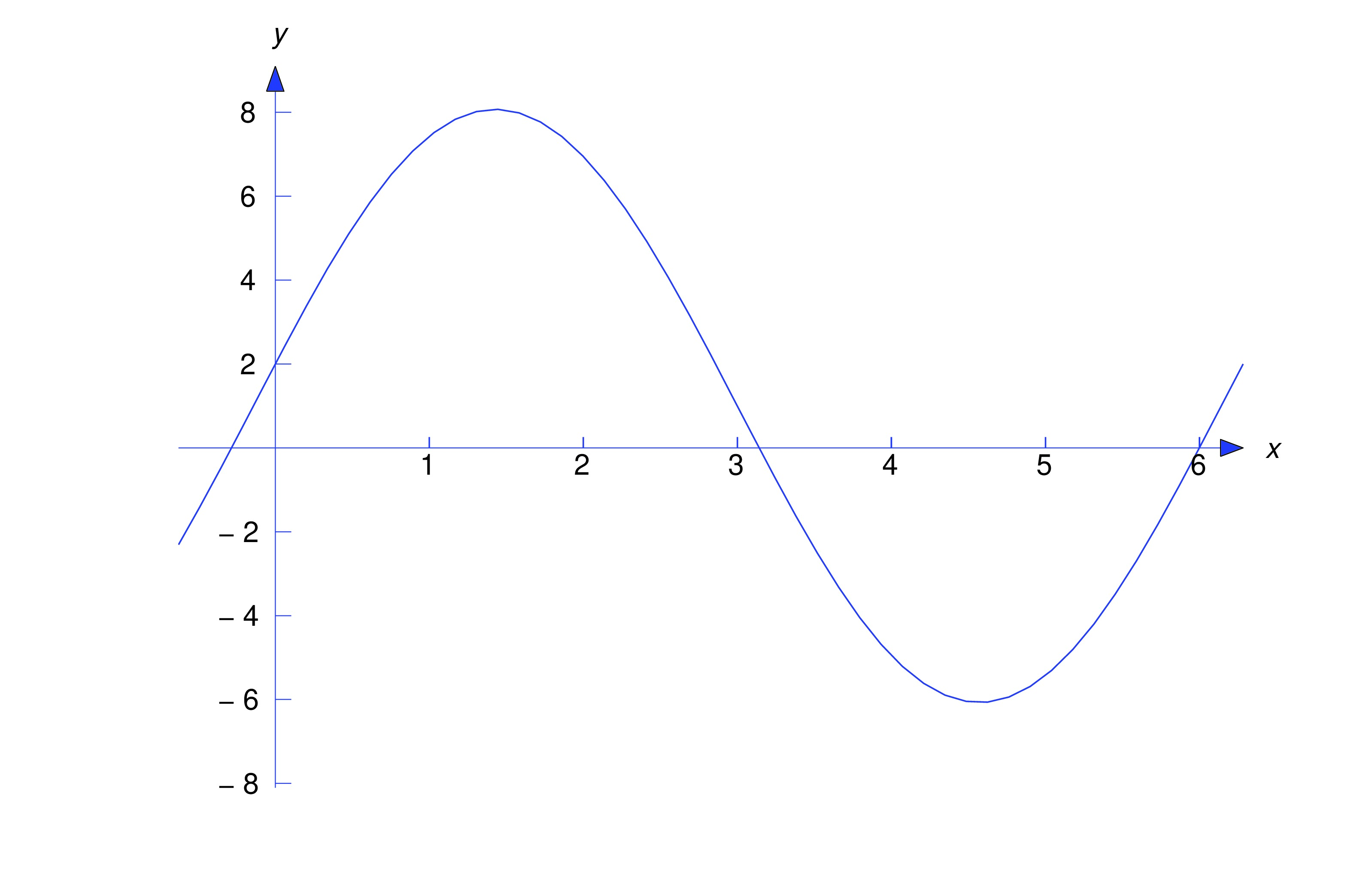
item:5.3.1b Imposing the initial condition in (eq:5.3.9) yields , so . Differentiating (eq:5.3.9) yields Imposing the initial condition here yields , so the solution of (eq:5.3.8) is The figure below shows a graph of this solution.
- (a)
- Find the general solution of
- (b)
- Solve the initial value problem
item:5.3.2a The characteristic polynomial of the complementary equation is , so and form a fundamental set of solutions of the complementary equation. To guess a form for a particular solution of (eq:5.3.10), we note that substituting a second degree polynomial into the left side of (eq:5.3.10) will produce another second degree polynomial with coefficients that depend upon , , and . The trick is to choose , , and so the polynomials on the two sides of (eq:5.3.10) have the same coefficients; thus, if so
Equating coefficients of like powers of on the two sides of the last equality yields
so , , and . Therefore is a particular solution of (eq:5.3.10) and Theorem thmtype:5.3.2 implies that is the general solution of (eq:5.3.10).
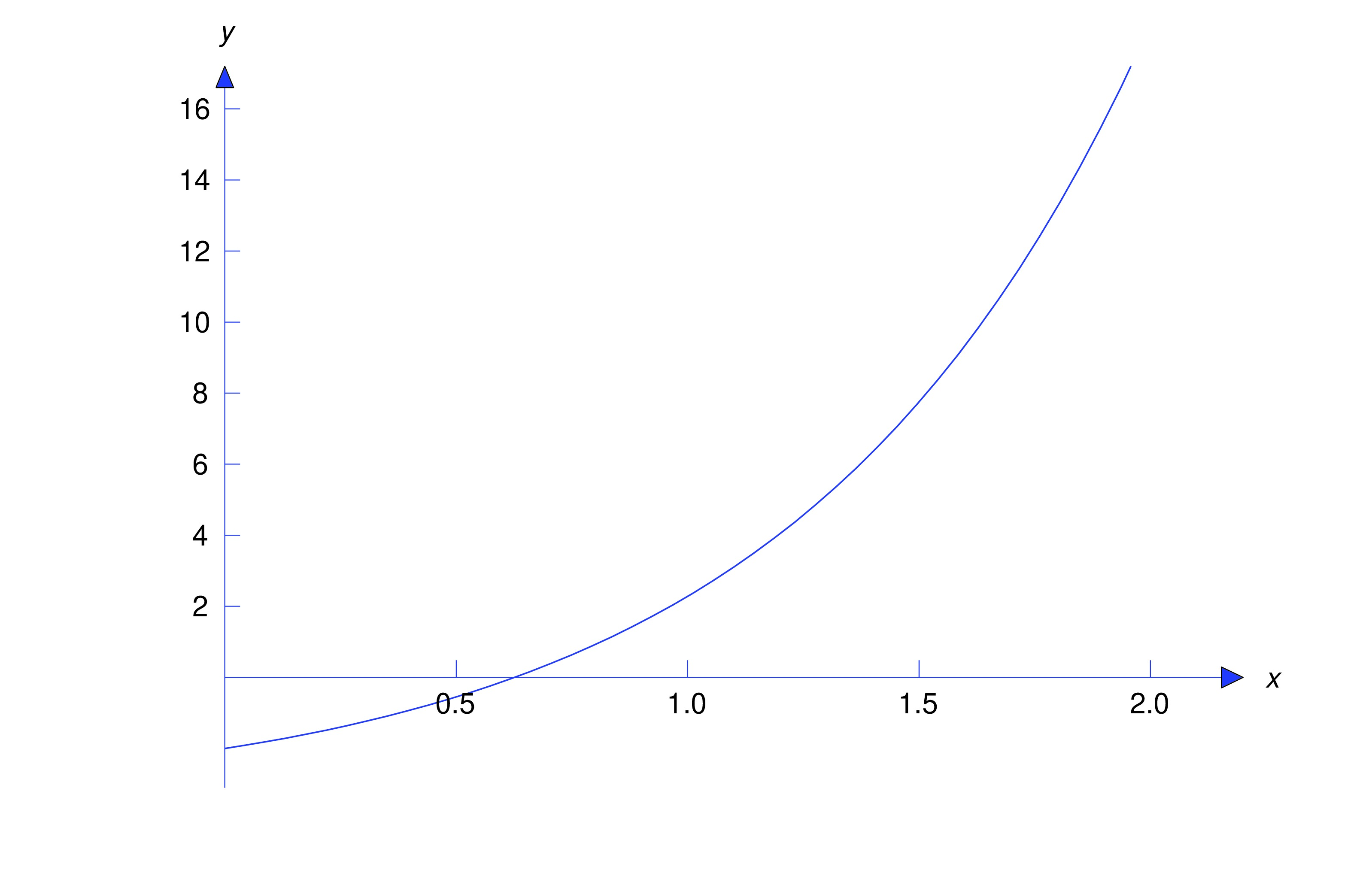
item:5.3.2b Imposing the initial condition in (eq:5.3.12) yields , so . Differentiating (eq:5.3.12) yields and imposing the initial condition here yields , so . Therefore the solution of (eq:5.3.11) is The figure below shows a graph of this solution.
Find the general solution of on and .
In Example example:5.1.3, we verified that and form a fundamental set of solutions of the complementary equation on and . To find a particular solution of (eq:5.3.13), we note that if , where is a constant then both sides of (eq:5.3.13) will be constant multiples of and we may be able to choose so the two sides are equal. This is true in this example, since if then if ; therefore, is a particular solution of (eq:5.3.13) on . Theorem thmtype:5.3.2 implies that the general solution of (eq:5.3.13) on and is
The Principle of Superposition
The next theorem enables us to break a nonhomogeous equation into simpler parts, find a particular solution for each part, and then combine their solutions to obtain a particular solution of the original problem.
The Principle of Superposition Suppose is a particular solution of on and is a particular solution of on . Then is a particular solution of on .
It's easy to generalize Theorem thmtype:5.3.3 to the equation
where thus, if is a particular solution of on for , , …, , then is a particular solution of (eq:5.3.14) on . Moreover, by a proof similar to the proof of Theorem thmtype:5.3.3 we can formulate the principle of superposition in terms of a linear equation written in the form that is, if is a particular solution of on and is a particular solution of on , then is a solution of on .
The function is a particular solution of on and is a particular solution of on . Use the principle of superposition to find a particular solution of on .
The right side in (eq:5.3.17) is the sum of the right sides in (eq:5.3.15) and (eq:5.3.16). Therefore the principle of superposition implies that is a particular solution of (eq:5.3.17).
Text Source
Trench, William F., "Elementary Differential Equations" (2013). Faculty Authored and Edited Books & CDs. 8. (CC-BY-NC-SA)
https://digitalcommons.trinity.edu/mono/8/
General Solution to a Nonhomogeneous Linear System of Ode's
Source: https://ximera.osu.edu/ode/main/nonHomogeneousLinear/nonHomogeneousLinear